2 Tutorial 1: Data Analysis with R
These notes have been updated and adapted for the course ECON 326: Introduction to Econometrics II, an undergraduate course at the University of British Columbia (UBC), 2026. These are the notes for the tutorial 1. This is an introduction to R and R Studio. ## Introduction to R and RStudio
This chapter introduces the basic workflow for working with R through RStudio. The goal is not only to learn commands, but also to develop good habits for writing clean, reproducible, and well-documented code.
2.0.1 Why use R?
R is one of the most widely used programming languages for data analysis in Economics and the Social Sciences. Its main advantages are:
- Open source: R is free and has an active community that constantly develops new tools.
- Versatility: it supports statistical and econometric analysis, data cleaning, visualization, and automation (including tasks like web scraping).
- Reproducibility: scripts and reports allow you to document and replicate results reliably.
- Labor market value: open-source programming languages are increasingly demanded across research and industry.
In this course we will treat R not as a “calculator”, but as a programming language: we will write code, create objects, use functions systematically, and build routines that scale to larger projects.
2.0.2 Key concepts (vocabulary of the course)
Before writing code, it is important to define the core terms that will appear throughout the course:
- RStudio: a Graphical User Interface (GUI) designed to make working with R easier.
- Objects: anything you store in memory (datasets, variables, lists, plots, models, etc.).
-
Functions: operations that take inputs and return outputs (e.g.,
mean(x),lm(y ~ x)). -
Packages: collections of functions grouped by purpose (e.g.,
dplyr,ggplot2,rio). - Scripts / Code: files containing the commands that define your analysis pipeline.
2.0.3 Learning resources
To learn R efficiently, you should rely on three types of resources: cheat sheets, forums, and structured books.
-
Cheat sheets: short summaries of commands and workflows.
Available at: https://www.rstudio.com/resources/cheatsheets/
-
Forums and websites:
- Stack Overflow: https://stackoverflow.com/questions/tagged/r
- Medium: https://preettheman.medium.com/awesome-tricks-every-r-coder-should-know-c4220cd2cfbc
- Posit Blog (formerly RStudio): https://posit.co/
-
Books:
- R for Data Science: https://r4ds.had.co.nz/
- Posit resources in Spanish: https://posit.co/resources/videos/
- Bookdown: https://bookdown.org/
2.0.4 RStudio interface
RStudio is a convenient “vehicle” for working with R. The interface usually displays four main panels, which help you organize your work:
- Scripts (Source): where you write and save code.
- Console: where R runs commands and prints results.
- Environment / History: where you see the objects created in memory.
- Files / Plots / Packages / Help: tools to navigate folders, view plots, manage packages, and read documentation.
A key takeaway is that most of your work should live in the Script, not in the Console. The Console is useful for quick checks, but scripts are what ensure reproducibility.
You can customize RStudio via: Tools → Global Options (font size, theme, layout, etc.). The purpose is to make your workflow as intuitive and efficient as possible.
2.1 Writing code: comments, structure and cleaning the environment
2.1.2 Outlines (code indexing)
RStudio allows you to structure scripts using headings. This creates an outline that helps navigation in long files.
- Open outline:
Ctrl + Shift + O
Headings can be hierarchical:
# The most important
## This is a bit less important
### This is a bit less important than the previous one
#### The least important
Keeping the outline updated is not optional: as the script grows, the outline becomes one of the main tools to navigate your code efficiently. If headings are outdated or inconsistent, the outline loses its usefulness and long scripts become harder to maintain.
2.1.3 Cleaning in R: environment vs console
When working in R, it is important to distinguish between two different things:
- The environment (memory): where R stores the objects you create (datasets, vectors, models, plots, etc.).
- The console (screen): where commands and results are printed.
Cleaning the environment is about deleting objects stored in memory.
Cleaning the console is only about making the screen look “clean” — it does not delete anything.
Remove all objects from the environment
Remove only one object
# rm(data1)2.2 Package installation, libraries and help
In R, most of the tools we use are contained in packages. A package is simply a collection of functions designed for a specific purpose (e.g., data cleaning, plotting, importing files, estimation).
A key distinction is the following:
- Packages are installed once on your computer.
- Packages must be loaded every time you open a new R session in order to use them.
This difference is crucial: many beginner errors come from confusing “installing” with “loading”.
2.2.1 Libraries
There are two standard ways to install packages in RStudio:
- Using the Packages tab in the bottom-right panel.
- Using commands directly in R.
install.packages("dplyr")Many packages at the same time:
install.packages(c("dplyr","ggplot2","rio"))Common error:
install.packages(dplyr, "ggplot2")In general, it is a good idea to install them at the beginning of your work, since we commonly use the same libraries when doing data analysis. With this function, we tell R to install the package if it is not installed (something typical when we switch computers):
if(!require(dplyr)) {install.packages("dplyr")}Load libraries:
If we want to see what is inside each package:
ls("package:dplyr", all = TRUE) #ls = list objectsImportant: the package must be installed once, but loaded every time it is used. There are often updates. To check and install them:
Alternatively, I can link a package to a function using ::. If I do this, it is not necessary to load the library in order to use that specific function. However, the recommended practice is to load all the libraries of the packages I will use at the beginning.
2.2.3 Useful Shortcuts
-
Esc: interrupt the current command -
Ctrl + s: save -
tab: autocomplete -
Ctrl + Enter: run line -
Ctrl + Shift + C: comment/uncomment -
<-: Alt + - / option + - -
%>%: Ctrl + Shift + M (pipe) -
Ctrl + l: clear console -
Ctrl + Alt + b: run everything up to here (the arrow keys in the console allow you to view the most recent commands used) -
Shift + lines: select multiple lines -
Ctrl + f: find/replace -
Ctrl + Up Arrow(in the console): view previously used commands
2.2.3.1 Identify the package of a function
Sometimes we want to know which package a given function belongs to. For that, check: https://sebastiansauer.github.io/finds_funs/ `
Note that a + sign appears in the console. In these cases, RStudio stops because you probably forgot a ) or a #. You must correct the error, run the code again, and then press Esc in the console to continue executing commands.
2.3 R Markdown - Reproducible research
R Markdown is one of the most useful tools in applied data analysis because it allows you to combine explanatory text with executable code in a single document. The key idea is simple:
You write the analysis once, and every time the data changes, you can re-run the document to automatically update tables, figures, and results.
This makes your work:
- Automatic: outputs are generated by code (not manually copied).
- Reproducible: anyone can re-run the document and obtain the same results.
- Well documented: results are always accompanied by explanations, interpretation, and methodology.
In practice, an R Markdown file (.Rmd) works like a hybrid between a report and a script: it contains written text (like a Word document) and chunks of code (like an R script). When you compile (“knit”) the file, R executes the code chunks and inserts the results (tables, plots, numbers) directly into the final report.
2.3.1 What can R Markdown produce?
An .Rmd file can generate many different types of outputs, such as:
-
Word reports (
.docx) -
PDF reports (
.pdf) -
HTML reports (
.html) - Presentations (slides)
- Dashboards (interactive documents)
More importantly, an .Rmd file can include all elements that typically appear in a data analysis:
- plain text explanations
- R code chunks
- tables
- plots
- regression output
- automatically updated statistics (means, SDs, p-values, etc.)
2.3.2 When is R Markdown especially useful?
R Markdown is particularly valuable in two common situations:
Routine reports
Example: a weekly report with updated descriptive statistics and graphs.
Instead of rewriting the report every week, you update the data and re-knit.Reports for subsets of a dataset
Example: a dataset contains several countries. You want one report per country.
With R Markdown, you can parameterize the report and automatically generate one output per country.
The general lesson is: if you are repeating work manually, it can probably be automated with R Markdown.
2.4 Basic concepts
To understand R Markdown, you need to distinguish the following components:
2.4.1 Markdown (.md)
Markdown is a simple plain-text language to format documents. For example:
-
# Titlecreates a section title -
**bold**produces bold text - lists, links, and images are easy to write
Markdown files have extension .md.
2.4.2 R Markdown (.Rmd)
R Markdown extends Markdown by allowing you to embed R code directly into the document. Files have extension .Rmd.
The most important feature is that R code is executed and its output is included in the report. This is what makes the document dynamic and reproducible.
2.4.3 knitr
knitr is the R package responsible for:
- reading the
.Rmdfile - identifying code chunks
- executing the R code
- inserting the results (tables/figures/output) into the document
In other words: knitr is the engine that turns the .Rmd file into a report.
2.4.4 Pandoc
Pandoc is the tool that converts the report into a final format such as PDF, Word, or HTML.
It takes the document produced by knitr and transforms it into a clean formatted file.
Pandoc is installed automatically with RStudio, so you do not need to install it manually.
2.4.5 Process (how everything works together)
The workflow is:
- You write text and R code in a single
.Rmddocument. -
knitrexecutes the code chunks. - Pandoc converts the final output into PDF/Word/HTML.

2.4.6 Your first R Markdown file
To create your first .Rmd document in RStudio:
- Go to: File → New File → R Markdown
- Choose the output format: report / presentation / dashboard
- Set the document title and author
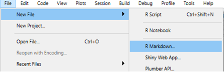
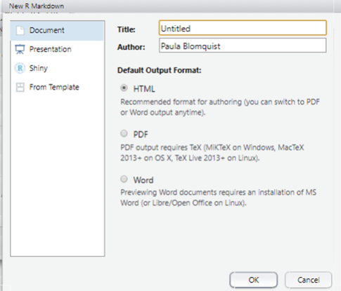
The most common starting point is a simple report that outputs to HTML or Word.
2.4.7 Working directory (critical detail)
A frequent source of confusion in R Markdown is the working directory.
The general rule is:
The working directory of an
.Rmdfile is the folder where the.Rmdfile is saved.
This means that if your .Rmd file is saved in a folder, R will look for datasets and external files in the same folder (unless you specify full paths).
For this course, we will keep things simple:
- store your data in the same folder as the .Rmd file
- avoid complicated paths until you gain familiarity
This is a best practice for beginners because it reduces file-loading errors.
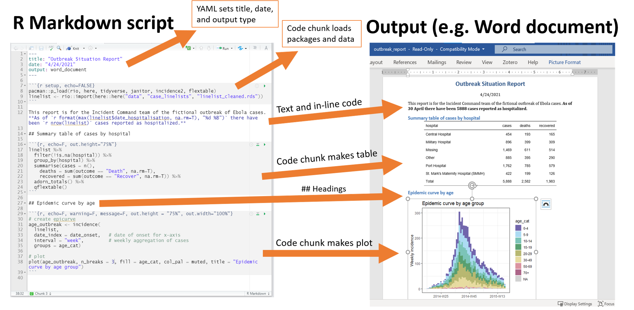
2.4.8 Components of an R Markdown file
An R Markdown file has three main components:
YAML header
A block at the top of the file containing metadata (title, author, output type).Markdown text
Where you write narrative explanations: motivation, steps, interpretation.Code chunks
Blocks of R code used for loading packages, importing data, transforming variables, estimating models, and generating plots.
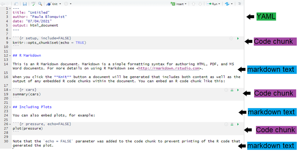
A code chunk looks like this:
A typical workflow is:
- YAML sets format + structure
- Markdown text explains what you are doing
- code chunks do the analysis and generate outputs
2.4.9 Why is this powerful?
In Word/Excel workflows, people often: - run regressions in one place, - copy results into a document, - manually update tables and plots.
This is slow and error-prone.
With R Markdown: - your report is generated directly from code, - results are always consistent with data, - there is no manual copy/paste.
That is why R Markdown is considered a core tool for reproducible research.
### Working directory
- The working directory of a
.Rmdfile is the folder where the file is saved. - Therefore, R will search for files in the same folder where the
.Rmdfile is stored. - For this exercise, we will simply keep the data we use in the same folder as the
.Rmdfile.
2.5 Object manipulation
2.5.0.1 Using R as a calculator / running commands
You can run commands in R in an interactive way, just like using a calculator. To do this, select the line(s) of code you want to execute and press:
-
Ctrl + Enter(Windows) -
Cmd + Enter(Mac)
This allows you to run commands separately (one line at a time or a selected block), without executing the entire script.
2+2 ## [1] 4
3*5^(1/2)## [1] 6.7082042.5.0.2 Running all instructions
To execute the entire script (i.e., run all commands in the file at once), you have several options:
- Click Source (top-right of the Script panel) to run the whole script.
- Use the menu: Code → Run Region → Run All.
- Shortcut:
Ctrl + Alt + R(Windows) /Cmd + Option + R(Mac)
Running the full script is useful when you want to reproduce the complete workflow from start to finish (e.g., cleaning data, generating tables, producing plots).
2+2 ; 3*5^(1/2)## [1] 4## [1] 6.708204
3+4 ## [1] 7
5*4 ## [1] 20
8/4 ## [1] 2
6^7## [1] 279936
6^77## [1] 8.272681e+59
log(10) ## [1] 2.302585
log(1)## [1] 0
sqrt(91) # raiz cuadrada## [1] 9.539392
round(7.3) # redondear## [1] 7Even large operations can be executed this way. For example, you can select and run a full block of code (data imports, transformations, loops, regressions, plots) instead of running commands one by one. This is especially useful when your analysis requires multiple steps that must be executed in the correct order.
## [1] 3292752213You can even work with complex numbers (imaginary numbers) in R.
In R, the imaginary unit is written as i, and complex numbers can be used in arithmetic operations just like real numbers.
Example:
2i+5i+sqrt(25i)## [1] 3.535534+10.53553i2.5.0.3 Object creation: assignment and functions
In R, we create objects using the assignment operator <-. This is one of the most important operations in the language, because almost everything we do in R consists of creating and transforming objects (vectors, datasets, models, plots, etc.).
It is also possible to assign values using =, but this is not recommended in general practice, since it can be confusing (especially inside functions). The recommended standard in most applied work is to use <-.
y <- 2 + 4
y
## [1] 62.6 Understanding Assignments and Functions in R
Assignments in R are silent operations. When we create an assignment, it stores the value but does not automatically display it in the console. To see the result of an assignment, we must explicitly call the object by typing its name or using the print() function.
While simple assignments are straightforward, the real power of R lies in generating assignments through functions. Functions are the central component of working with R. Some functions come pre-installed with the base R installation, while others must be obtained from external packages. Additionally, users can write their own custom functions. Functions are typically written with parentheses, such as filter(). In some cases, functions are associated with specific packages and are referenced using the double colon notation, for example dplyr::filter().
Let’s explore how functions work through several examples. First, we can apply a simple mathematical function:
sqrt(49)## [1] 7This calculates the square root of 49. We can also apply functions to datasets. For instance, we can obtain summary statistics for a variable within a dataset:
summary(mtcars$mpg)## Min. 1st Qu. Median Mean 3rd Qu. Max.
## 10.40 15.43 19.20 20.09 22.80 33.90The mtcars dataset comes pre-installed with R and contains information about various car models. To see other datasets that come bundled with R, we can use the data() function:
data()2.6.1 Working with Vectors and Arithmetic Functions
We can create objects by assigning values to them and then combine these objects into vectors. A vector is a fundamental data structure in R that contains elements of the same type:
x <- 2
y <- 3
z <- c(x, y)
z
## [1] 2 3Here, we create two individual numeric objects (x and y) and then combine them into a vector z using the concatenate function c(). Once we have a vector, we can apply various statistical functions to it:
mean(z)## [1] 2.5
median(z)## [1] 2.5These functions calculate the arithmetic mean and median of the values in the vector, respectively.
2.6.2 Creating Relationships Between Objects
We can create new objects based on calculations performed on existing objects. For example, we can store the mean of a vector as a new object:
w <- mean(z)We can also create objects through arithmetic operations:
a <- 3 + 10
b <- 2 * 4
R allows us to perform logical comparisons between objects:
a > b## [1] TRUEThis returns a logical value (TRUE or FALSE) indicating whether a is greater than b.
2.6.3 The Silent Nature of Assignments
As mentioned earlier, assignments do not produce output unless we explicitly request it. To display the contents of an object, we simply type its name or use the print() function:
a## [1] 13
b## [1] 8
# alternatively, use print
print(a)
## [1] 13
print(b)## [1] 82.6.4 Building Complex Objects from Functions
We can build more complex objects by combining multiple operations. For instance, we can create a vector from previously defined objects and calculate its mean:
## [1] 10.5
promedio## [1] 10.5Let’s work through another example where we calculate the mean of two values:
## [1] 3.5To clear our workspace and remove specific objects, we can use the rm() function:
## Warning in rm(promedio): object 'promedio' not foundThe first command removes all objects from the environment, while the second removes a specific object.
2.6.5 Working with Real Data: Education and Income Example
Proper spacing and organization of code is essential for readability and maintenance. Let’s create two vectors representing education (in years) and income for ten individuals using the concatenate function c():
educ <- c(8, 12, 8, 11, 16, 14, 8, 10, 14, 12)
ingreso <- c(325, 415, 360, 380, 670, 545, 350, 420, 680, 465)
Once we have these vectors, we can calculate various descriptive statistics. We can compute the mean income, the standard deviation of income, and the correlation between education and income:
mean(ingreso)## [1] 461## [1] 129.1382## [1] 0.9110521
coreduing <- cor(educ, ingreso)The mean provides the average income, the standard deviation measures the dispersion of income values around the mean, and the correlation coefficient quantifies the strength and direction of the linear relationship between education and income.
2.6.6 Visualizing the Relationship
To visually examine the relationship between education and income, we can create a scatter plot:
plot(educ, ingreso)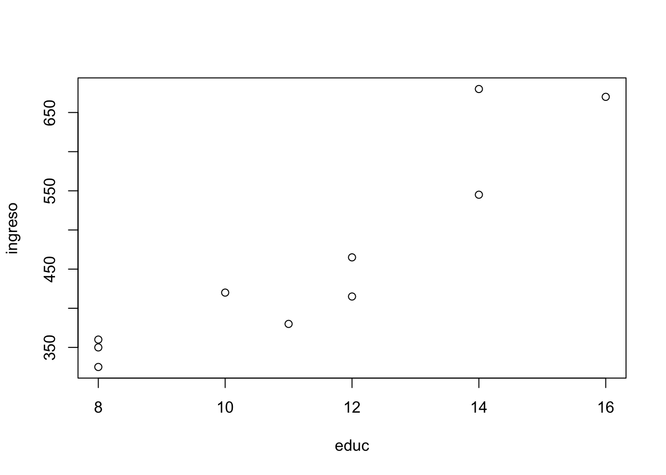
This produces a graph with education on the x-axis and income on the y-axis, allowing us to see the pattern of association between these two variables.
2.6.7 Estimating a Linear Regression Model
Finally, we can formally model the relationship between education and income using linear regression. The lm() function estimates a linear model where income is the dependent variable and education is the independent variable:
lm(ingreso ~ educ)##
## Call:
## lm(formula = ingreso ~ educ)
##
## Coefficients:
## (Intercept) educ
## -8.71 41.57This function returns the estimated coefficients for the linear model, providing us with the intercept and the slope coefficient for education. The slope coefficient indicates how much income is expected to change for each additional year of education.
2.7 Object Naming and Types
2.7.1 Naming Objects
The following exercise helps us understand the rules for valid variable names in R.
Exercise: Valid Variable Names
Consider the following examples. Which of these are valid variable names in R?
# min_height      # Valid: uses underscore
# max.height      # Valid: uses dot
# _age            # Invalid: starts with underscore
# .mass           # Valid: starts with dot (but creates hidden variable)
# MaxLength       # Valid: uses camel case
# Min-length      # Invalid: uses hyphen (minus sign)
# 2widths         # Invalid: starts with number
# Calsius2kelvin  # Valid: number in middle is allowed
In R, variable names must follow these rules: they can contain letters, numbers, dots, and underscores, but they must start with a letter or a dot (if starting with a dot, the second character cannot be a number). Variable names cannot contain spaces or special characters like hyphens, and they cannot start with numbers or underscores.
2.7.2 Types of Objects
2.7.2.1 Vectors
R operates component by component, which makes it very straightforward to work with vectors and matrices. Vectors are one-dimensional arrays that can hold numeric data, character data, or logical data, but all elements must be of the same type.
To create a vector, we use the c() function (which stands for “concatenate” or “combine”):
Let’s examine what happens when we add vectors together:
z <- x + y## Warning in x + y: longer object length is not a multiple of shorter object
## length
z## [1] 7 9 11 10 12Now, let’s consider two vectors of different lengths:
We can check the length of each vector using the length() function:
length(x)## [1] 4
length(y)## [1] 3What happens when we try to add vectors of different lengths?
z <- x + y## Warning in x + y: longer object length is not a multiple of shorter object
## length
z## [1] 2 4 6 5IMPORTANT: In this case, R performs the operation anyway, but it gives us a warning that the lengths differ. R uses “vector recycling,” where the shorter vector is repeated to match the length of the longer vector. A crucial characteristic of vectors is that they can only concatenate elements of the same type; otherwise, R will coerce all elements to a common type (usually character if there’s a mix).
Let’s explore more vector operations:
x <- rep(1.5:9.5, 4)  # generates repetitions of the defined values
y <- c(20:30)
x1 <- c(1, 2)
x2 <- c(3, 4)
x3 <- c(x1, x2)
x4 <- c(c(1, 2), c(3, 4))
2.7.2.1.1 Subsetting Vectors
We can extract specific elements from a vector using square bracket notation:
y[3] # get the third element## [1] 22
y[2:4] # get elements 2 through 4## [1] 21 22 23
y[4:2] # get elements in reverse order (4, 3, 2)## [1] 23 22 21
y[c(2, 6)] # get elements 2 and 6## [1] 21 25
y[c(2, 16)] # attempt to get element 16 (returns NA if out of bounds)## [1] 21 NA2.7.2.2 Matrices
Matrices are two-dimensional arrays where all elements must be of the same type. They are particularly useful for mathematical operations and organizing data in rows and columns.
2.7.2.2.1 Defining Matrices
The general syntax for creating a matrix is:
my.matrix <- matrix(vector,
                    ncol = num_columns,
                    nrow = num_rows,
                    byrow = logical_value,
                    dimnames = list(vector_row_names,
                                   vector_column_names))
To create matrices, we use the matrix() function:
While it is not necessary to explicitly write data=, doing so improves code readability and makes the intent clearer.
x## [,1] [,2]
## [1,] 1 3
## [2,] 2 4
x1## [,1] [,2]
## [1,] 1 3
## [2,] 2 4Note that by DEFAULT, R fills the matrix column by column. We can explicitly specify that we want to fill the matrix row by row using the byrow argument:
## Warning in matrix(data = c(1:4), nrow = 3, ncol = 2, byrow = TRUE): data
## length [4] is not a sub-multiple or multiple of the number of rows [3]
y## [,1] [,2]
## [1,] 1 2
## [2,] 3 4
## [3,] 1 2We can determine the dimensions of a matrix using the dim() function:
dim(y)## [1] 3 2
dim(y)[1] # number of rows## [1] 3
dim(y)[2] # number of columns## [1] 2## [,1] [,2]
## [1,] 1 2
## [2,] 3 4If the vector is shorter than the matrix dimensions, R will recycle the values to fill the matrix:
## Warning in matrix(c(1, 2, 3, 4), nrow = 2, ncol = 3, byrow = 2): data
## length [4] is not a sub-multiple or multiple of the number of columns [3]
y## [,1] [,2] [,3]
## [1,] 1 2 3
## [2,] 4 1 2Note that the order in any matrix is always rows × columns. We can also omit either the number of rows or columns, and R will calculate the missing dimension:
##      [,1] [,2]
## [1,]    1    2
## [2,] 3 4When creating empty matrices, we must define the dimensions:
y <- matrix(nrow = 3, ncol = 3)
y  # useful for loops where we fill values iteratively
## [,1] [,2] [,3]
## [1,] NA NA NA
## [2,] NA NA NA
## [3,] NA NA NA2.7.2.2.2 Naming Rows and Columns
We can assign names to rows and columns directly in the matrix() function:
##    Y1 Y2
## X1  1  3
## X2  2  4
Alternatively, we can use the colnames() and rownames() functions:
##    Variable 1 Variable 2
## a1          1          3
## a2          2          4
2.7.2.2.3 Adding Rows or Columns to a Matrix
Let’s create a new vector to add to our matrix:
w <- c(5, 6)We can combine matrices and vectors using rows (note that the vector name becomes the row name):
z <- rbind(x, w)
z
## Variable 1 Variable 2
## a1 1 3
## a2 2 4
## w 5 6We can also combine using columns:
z <- cbind(x, w)
z
## Variable 1 Variable 2 w
## a1 1 3 5
## a2 2 4 6What happens if they have different numbers of rows and/or columns? R will recycle the shorter vector or observation to match the longer dimension:
##      [,1] [,2] [,3]
## [1,]    1    4    7
## [2,]    2    5    8
## [3,]    3    6    9
y <- c(5, 6)
y
## [1] 5 6
z <- rbind(x, y)## Warning in rbind(x, y): number of columns of result is not a multiple of
## vector length (arg 2)
z## [,1] [,2] [,3]
## 1 4 7
## 2 5 8
## 3 6 9
## y 5 6 52.7.2.2.4 Converting Vectors to Matrices
We can convert a vector to a matrix by assigning dimensions:
x <- 1:10
x
## [1] 1 2 3 4 5 6 7 8 9 10## [,1] [,2] [,3] [,4] [,5]
## [1,] 1 3 5 7 9
## [2,] 2 4 6 8 102.7.2.2.5 Transposing Matrices
We can transpose a matrix (swap rows and columns) using the t() function:
##      [,1] [,2] [,3]
## [1,]    1    2    3
## [2,]    4    5    6
## [3,]    7    8    9
2.7.2.2.6 Subsetting Matrices
We can extract specific elements, rows, or columns from a matrix. For example, to get the second and fourth elements of the second row:
M <- matrix(1:8, nrow = 2)
M
## [,1] [,2] [,3] [,4]
## [1,] 1 3 5 7
## [2,] 2 4 6 8
M[1, 1] # element in first row, first column## [1] 1
M[1, ] # entire first row## [1] 1 3 5 7
M[, 2] # entire second column## [1] 3 4
M[2, c(2, 4)] # second and fourth elements of the second row## [1] 4 8Matrix subsetting uses the format [row, column], where leaving either position blank returns all rows or all columns, respectively.
2.8 Arrays
Arrays are multidimensional data structures that extend the concept of matrices. While matrices are two-dimensional, arrays can have three or more dimensions. They are particularly useful when working with data that naturally has multiple dimensions, such as time series data across different regions and variables.
2.8.1 Creating Arrays
The basic syntax for creating an array is: array(data, dim, dimnames)
## , , 1
##
##      [,1] [,2] [,3] [,4]
## [1,]    1    3    5    7
## [2,]    2    4    6    8
##
## , , 2
##
## [,1] [,2] [,3] [,4]
## [1,] 9 11 13 15
## [2,] 10 12 14 16
##
## , , 3
##
## [,1] [,2] [,3] [,4]
## [1,] 17 19 21 23
## [2,] 18 20 22 24The array above has dimensions 2 × 4 × 3, meaning it has 2 rows, 4 columns, and 3 “layers” or levels in the third dimension.
2.8.2 Adding Dimension Names
Dimension names make arrays much easier to interpret and work with:
# Define names for each dimension
dim1 <- c("row1", "row2")
dim2 <- c("col1", "col2", "col3", "col4")
dim3 <- c("level1", "level2", "level3")

# Create array with named dimensions
my_array <- array(1:24, c(2, 4, 3),
                  dimnames = list(dim1, dim2, dim3))
my_array
## , , level1
##
## col1 col2 col3 col4
## row1 1 3 5 7
## row2 2 4 6 8
##
## , , level2
##
## col1 col2 col3 col4
## row1 9 11 13 15
## row2 10 12 14 16
##
## , , level3
##
## col1 col2 col3 col4
## row1 17 19 21 23
## row2 18 20 22 242.8.3 Accessing Array Elements
Arrays can be subset using square brackets, similar to matrices but with additional dimensions:
# Access a single element: row 1, column 2, level 3
my_array[1, 2, 3]
## [1] 19
# Access entire slices
my_array[, , 1]  # All of level 1
## col1 col2 col3 col4
## row1 1 3 5 7
## row2 2 4 6 8
my_array[1, , ] # All of row 1 across all levels## level1 level2 level3
## col1 1 9 17
## col2 3 11 19
## col3 5 13 21
## col4 7 15 23
# Access by dimension names
my_array["row1", "col2", "level3"]
## [1] 192.9 Lists
Lists are R’s most flexible data structure. Unlike vectors, which must contain elements of the same type, lists can contain elements of different types, including other lists, vectors, matrices, dataframes, and even functions.
2.9.1 Creating Lists
# Create a heterogeneous list
my_list <- list(
  numbers = c(1, 2, 3),
  text = "Hello R",
  matrix = matrix(1:6, nrow = 2),
  flag = TRUE
)

my_list
## $numbers
## [1] 1 2 3
##
## $text
## [1] "Hello R"
##
## $matrix
## [,1] [,2] [,3]
## [1,] 1 3 5
## [2,] 2 4 6
##
## $flag
## [1] TRUE2.9.2 Accessing List Components
Lists have three main ways to access their components:
# Method 1: Double brackets [[ ]] - extracts the element itself
my_list[[1]]  # Returns the numeric vector
## [1] 1 2 3
# Method 2: Dollar sign $ - access by name
my_list$text  # Returns "Hello R"
## [1] "Hello R"
# Method 3: Single brackets [ ] - returns a sublist
my_list[1]    # Returns a list containing the first element
## $numbers
## [1] 1 2 3
# Accessing nested elements
my_list[[3]][1, 2]  # Second element of first row in the matrix
## [1] 32.9.3 Adding and Removing List Elements
# Adding new components
my_list$new_vector <- c(10, 20, 30)

# Removing components (set to NULL)
my_list$flag <- NULL

# View updated structure
str(my_list)
## List of 4
## $ numbers : num [1:3] 1 2 3
## $ text : chr "Hello R"
## $ matrix : int [1:2, 1:3] 1 2 3 4 5 6
## $ new_vector: num [1:3] 10 20 302.10 Data Frames
Data frames are the workhorse data structure for statistical analysis in R. They are similar to matrices but can contain columns of different types, making them perfect for representing datasets where variables may be numeric, character, or logical.
2.10.1 Creating Data Frames
# Create a data frame
df <- data.frame(
  ID = 1:5,
  Name = c("Alice", "Bob", "Charlie", "Diana", "Eve"),
  Age = c(25, 30, 35, 28, 32),
  Employed = c(TRUE, TRUE, FALSE, TRUE, TRUE)
)

df
## ID Name Age Employed
## 1 1 Alice 25 TRUE
## 2 2 Bob 30 TRUE
## 3 3 Charlie 35 FALSE
## 4 4 Diana 28 TRUE
## 5 5 Eve 32 TRUE2.10.2 Exploring Data Frame Structure
# View structure
str(df)
## 'data.frame': 5 obs. of 4 variables:
## $ ID : int 1 2 3 4 5
## $ Name : chr "Alice" "Bob" "Charlie" "Diana" ...
## $ Age : num 25 30 35 28 32
## $ Employed: logi TRUE TRUE FALSE TRUE TRUE
# Dimensions
dim(df)
## [1] 5 4
nrow(df)## [1] 5
ncol(df)## [1] 4
# Column names
names(df)
## [1] "ID" "Name" "Age" "Employed"
colnames(df)## [1] "ID" "Name" "Age" "Employed"
# Summary statistics
summary(df)
## ID Name Age Employed
## Min. :1 Length:5 Min. :25 Mode :logical
## 1st Qu.:2 Class :character 1st Qu.:28 FALSE:1
## Median :3 Mode :character Median :30 TRUE :4
## Mean :3 Mean :30
## 3rd Qu.:4 3rd Qu.:32
## Max. :5 Max. :35
# First and last rows
head(df, 3)
## ID Name Age Employed
## 1 1 Alice 25 TRUE
## 2 2 Bob 30 TRUE
## 3 3 Charlie 35 FALSE
tail(df, 2)## ID Name Age Employed
## 4 4 Diana 28 TRUE
## 5 5 Eve 32 TRUE2.10.3 Subsetting Data Frames
Data frames combine the subsetting behavior of both matrices and lists:
# Accessing columns
df$Name           # By name with $
## [1] "Alice" "Bob" "Charlie" "Diana" "Eve"
df[, "Age"] # By name with brackets## [1] 25 30 35 28 32
df[, 3] # By position## [1] 25 30 35 28 32
# Accessing rows
df[2, ]           # Second row
## ID Name Age Employed
## 2 2 Bob 30 TRUE
# Accessing specific cells
df[2, 3]          # Row 2, Column 3
## [1] 30
df[2, "Age"] # Same, using column name## [1] 30
# Subsetting with conditions
df[df$Age > 28, ]                    # Rows where Age > 28
## ID Name Age Employed
## 2 2 Bob 30 TRUE
## 3 3 Charlie 35 FALSE
## 5 5 Eve 32 TRUE
df[df$Employed == TRUE, c("Name", "Age")] # Employed people's names and ages## Name Age
## 1 Alice 25
## 2 Bob 30
## 4 Diana 28
## 5 Eve 322.10.4 Tibbles: Modern Data Frames
The tibble package (part of tidyverse) provides an enhanced version of data frames:
library(tibble)

# Create a tibble
tb <- tibble(
  ID = 1:5,
  Name = c("Alice", "Bob", "Charlie", "Diana", "Eve"),
  Age = c(25, 30, 35, 28, 32),
  Employed = c(TRUE, TRUE, FALSE, TRUE, TRUE)
)

tb
## # A tibble: 5 × 4
## ID Name Age Employed
## <int> <chr> <dbl> <lgl>
## 1 1 Alice 25 TRUE
## 2 2 Bob 30 TRUE
## 3 3 Charlie 35 FALSE
## 4 4 Diana 28 TRUE
## 5 5 Eve 32 TRUE
# Tibbles have better printing and more consistent behavior2.11 Data Types and Type Checking
Understanding data types is crucial for avoiding errors and writing robust R code.
2.11.1 Main Data Types
# Character
char_var <- "Hello"
class(char_var)
## [1] "character"
# Numeric (double precision)
num_var <- 3.14
class(num_var)
## [1] "numeric"
# Integer
int_var <- 42L
class(int_var)
## [1] "integer"
# Logical
log_var <- TRUE
class(log_var)
## [1] "logical"
# Complex
complex_var <- 3 + 2i
class(complex_var)
## [1] "complex"2.11.2 Type Checking Functions
x <- 42

# Specific type checks
is.numeric(x)
## [1] TRUE
is.integer(x)## [1] FALSE
is.character(x)## [1] FALSE
is.logical(x)## [1] FALSE
# Convert x to integer
x_int <- as.integer(x)
is.integer(x_int)
## [1] TRUE2.11.3 Type Coercion
When R combines different types, it follows a coercion hierarchy: logical → integer → numeric → complex → character
# Combining logical and numeric
c(TRUE, 1, 2)  # TRUE becomes 1
## [1] 1 1 2
# Combining numeric and character
c(1, 2, "three")  # Numbers become characters
## [1] "1" "2" "three"
# Explicit coercion
as.character(42)
## [1] "42"
as.numeric("3.14")## [1] 3.14
as.logical(1) # Non-zero numbers become TRUE## [1] TRUE2.11.4 Missing Values
R uses NA (Not Available) to represent missing values.
## [1] FALSE FALSE TRUE FALSE TRUE## [1] 2
# Removing missing values
x[!is.na(x)]
## [1] 1 2 4
na.omit(x)## [1] 1 2 4
## attr(,"na.action")
## [1] 3 5
## attr(,"class")
## [1] "omit"
# Many functions have na.rm parameter
mean(x)              # Returns NA
## [1] NA
mean(x, na.rm = TRUE) # Calculates mean ignoring NAs## [1] 2.3333332.12 If-Else Statements
# Basic if statement
x <- 10

if (x > 5) {
  print("x is greater than 5")
}
## [1] "x is greater than 5"
# If-else
x <- 3

if (x > 5) {
  print("x is greater than 5")
} else {
  print("x is less than or equal to 5")
}
## [1] "x is less than or equal to 5"
# If-else if-else chain
score <- 75

if (score >= 90) {
  grade <- "A"
} else if (score >= 80) {
  grade <- "B"
} else if (score >= 70) {
  grade <- "C"
} else {
  grade <- "F"
}

grade
## [1] "C"2.13 Vectorized If-Else: ifelse()
The ifelse() function is vectorized, making it perfect for applying conditions to entire vectors:
# Create a vector of test scores
scores <- c(92, 75, 88, 65, 95, 70)

# Assign grades using ifelse
grades <- ifelse(scores >= 80, "Pass", "Fail")
grades
## [1] "Pass" "Fail" "Pass" "Fail" "Pass" "Fail"
# Nested ifelse for multiple conditions
detailed_grades <- ifelse(scores >= 90, "A",
                   ifelse(scores >= 80, "B",
                   ifelse(scores >= 70, "C", "F")))
detailed_grades
## [1] "A" "C" "B" "F" "A" "C"2.13.1 Functions
Functions are reusable blocks of code that perform specific tasks. They are fundamental to writing clean, maintainable code.
2.13.2 Creating Functions
# Basic function structure
square <- function(x) {
  result <- x^2
  return(result)
}

square(4)
## [1] 16
square(1:5)## [1] 1 4 9 16 252.13.3 Functions with Multiple Arguments
# Function with default parameter values
power <- function(base, exponent = 2) {
  result <- base^exponent
  return(result)
}

power(3)      # Uses default exponent = 2
## [1] 9
power(3, 3) # Explicit exponent## [1] 27
power(2, exponent = 4) # Named argument## [1] 162.13.4 Practical Example: Statistical Summary Function
# Create a function that returns multiple statistics
summary_stats <- function(x, na.rm = TRUE) {
  list(
    mean = mean(x, na.rm = na.rm),
    median = median(x, na.rm = na.rm),
    sd = sd(x, na.rm = na.rm),
    min = min(x, na.rm = na.rm),
    max = max(x, na.rm = na.rm),
    n = length(x),
    n_missing = sum(is.na(x))
  )
}

# Test the function
test_data <- c(1, 2, 3, NA, 5, 6, 7, NA, 9, 10)
summary_stats(test_data)
## $mean
## [1] 5.375
##
## $median
## [1] 5.5
##
## $sd
## [1] 3.248626
##
## $min
## [1] 1
##
## $max
## [1] 10
##
## $n
## [1] 10
##
## $n_missing
## [1] 22.14 Loops and Iteration
2.14.1 For Loops
For loops iterate over a sequence of values:
## [1] "Iteration 1"
## [1] "Iteration 2"
## [1] "Iteration 3"
## [1] "Iteration 4"
## [1] "Iteration 5"
# Iterating over vector elements
fruits <- c("apple", "banana", "cherry")

for (fruit in fruits) {
  print(paste("I like", fruit))
}
## [1] "I like apple"
## [1] "I like banana"
## [1] "I like cherry"
# Building results in a loop
squares <- numeric(10)
for (i in 1:10) {
  squares[i] <- i^2
}
squares
## [1] 1 4 9 16 25 36 49 64 81 1002.14.2 While Loops
While loops continue until a condition becomes FALSE:
# Basic while loop
counter <- 1

while (counter <= 5) {
  print(paste("Counter is", counter))
  counter <- counter + 1
}
## [1] "Counter is 1"
## [1] "Counter is 2"
## [1] "Counter is 3"
## [1] "Counter is 4"
## [1] "Counter is 5"
# Practical example: finding first value above threshold
x <- 1
while (2^x < 1000) {
  x <- x + 1
}
print(paste("2^", x, "=", 2^x, "is the first power of 2 above 1000"))
## [1] "2^ 10 = 1024 is the first power of 2 above 1000"2.14.3 Apply Family Functions
The apply family provides functional programming alternatives to loops. They are often faster and more concise.
2.14.4 lapply: Apply Function to List/Vector
lapply always returns a list:
# Apply function to each element
numbers <- list(a = 1:5, b = 6:10, c = 11:15)

# Calculate mean of each element
lapply(numbers, mean)
## $a
## [1] 3
##
## $b
## [1] 8
##
## $c
## [1] 13
# Using anonymous function
lapply(numbers, function(x) x^2)
## $a
## [1] 1 4 9 16 25
##
## $b
## [1] 36 49 64 81 100
##
## $c
## [1] 121 144 169 196 225
# Practical example: read multiple files
# file_names <- c("data1.csv", "data2.csv", "data3.csv")
# data_list <- lapply(file_names, read.csv)
2.14.5 sapply: Simplified Apply
sapply tries to simplify the result to a vector or matrix:
# Same operation, simplified output
sapply(numbers, mean)
## a b c
## 3 8 13## a b c
## 55 330 855
# When result can't be simplified, returns list like lapply
sapply(numbers, function(x) c(min = min(x), max = max(x)))## a b c
## min 1 6 11
## max 5 10 152.14.6 vapply: Type-Safe Apply
vapply requires you to specify the output type, making it safer and sometimes faster:
##  a  b  c
##  3  8 13
# For multiple return values
vapply(numbers, function(x) c(mean = mean(x), sd = sd(x)),
       FUN.VALUE = numeric(2))
## a b c
## mean 3.000000 8.000000 13.000000
## sd 1.581139 1.581139 1.581139
# Type safety prevents errors
# This would error if we tried to return character when numeric specified
2.15 Comparison and Best Practices
# Create example data
my_list <- list(
  group1 = rnorm(100, mean = 10, sd = 2),
  group2 = rnorm(100, mean = 15, sd = 3),
  group3 = rnorm(100, mean = 20, sd = 4)
)

# lapply: Always returns list
result_l <- lapply(my_list, summary)
class(result_l)
## [1] "list"## [1] "numeric"
# vapply: Type-safe, better for production code
result_v <- vapply(my_list, mean, FUN.VALUE = numeric(1))
class(result_v)
## [1] "numeric"Best Practices:
- Use lapply when you need a list output or when applying complex functions
- Use sapply for interactive analysis when you want simplified output
- Use vapply in production code or packages where type safety is important
2.16 Practical Applications
2.16.1 Example 1: Data Cleaning Pipeline
# Create sample data with issues
messy_data <- data.frame(
  id = 1:6,
  value = c(10, 20, NA, 40, 50, 60),
  category = c("A", "B", "A", "C", "B", "A"),
  valid = c(TRUE, TRUE, FALSE, TRUE, TRUE, TRUE)
)

# Function to clean and summarize
clean_and_summarize <- function(df) {
  # Remove invalid rows
  df_clean <- df[df$valid == TRUE, ]

  # Remove missing values
  df_clean <- df_clean[!is.na(df_clean$value), ]

  # Calculate summary by category
  categories <- unique(df_clean$category)
  results <- lapply(categories, function(cat) {
    subset_data <- df_clean[df_clean$category == cat, "value"]
    c(
      category = cat,
      mean = mean(subset_data),
      n = length(subset_data)
    )
  })

  # Combine into data frame
  do.call(rbind, results)
}

clean_and_summarize(messy_data)
## category mean n
## [1,] "A" "35" "2"
## [2,] "B" "35" "2"
## [3,] "C" "40" "1"2.16.2 Example 2: Simulation Study
# Function to simulate and analyze data
simulate_experiment <- function(n_samples, effect_size) {
  # Generate data
  control <- rnorm(n_samples, mean = 100, sd = 15)
  treatment <- rnorm(n_samples, mean = 100 + effect_size, sd = 15)

  # Perform t-test
  test_result <- t.test(treatment, control)

  # Return key results
  list(
    effect_size = effect_size,
    p_value = test_result$p.value,
    significant = test_result$p.value < 0.05
  )
}

# Run simulations for different effect sizes
effect_sizes <- seq(0, 10, by = 2)
simulation_results <- lapply(effect_sizes, function(es) {
  simulate_experiment(n_samples = 50, effect_size = es)
})

# Convert to data frame for easy viewing
results_df <- do.call(rbind, lapply(simulation_results, as.data.frame))
results_df
## effect_size p_value significant
## 1 0 0.0330407708 TRUE
## 2 2 0.4825550352 FALSE
## 3 4 0.3648947905 FALSE
## 4 6 0.0078056580 TRUE
## 5 8 0.2618240342 FALSE
## 6 10 0.0001524551 TRUE2.17 Summary
This tutorial covered essential advanced R programming concepts:
- Arrays: Multidimensional data structures for complex data
- Lists: Flexible containers for heterogeneous data
- Data Frames & Tibbles: Core structures for statistical data analysis
- Data Types: Understanding and working with different types
- Conditionals: Making decisions in code with if-else and ifelse
- Functions: Creating reusable, modular code
- Loops: For and while loops for iteration
- Apply Functions: Functional programming with lapply, sapply, and vapply
These tools form the foundation for efficient data analysis and statistical programming in R. Mastering them will enable you to write cleaner, more maintainable, and more efficient R code.
2.17.1 Key Takeaways
- Choose the right data structure: vectors for homogeneous data, lists for heterogeneous, data frames for tabular data
- Prefer vectorized operations over loops when possible
- Write functions to avoid repeating code
- Use apply functions instead of for loops for cleaner functional code
- Check and handle missing values explicitly
- Use type-safe functions (like vapply) in production code
2.1.1 Comments
Good code is code that other people (including “future you”) can understand. Comments are essential to explain why you do something, not only what you do.
To write comments in R scripts, use
#. To comment multiple lines at once use:Ctrl + Shift + C(Windows)Cmd + Shift + C(Mac)A very useful reference for best practices is:
Code and Data for the Social Sciences: A Practitioner’s Guide