3 Tutorial 2: Simple linear Regression
3.1 Problem 1: Simple Linear Regression with Intercept
In Tutorial 1 we ran lm() and got a slope and an intercept. This tutorial asks: where do those numbers come from, and what do they optimize?
The goal of simple linear regression is to summarize the relationship between two variables — education and wages, match rates and 401(k) participation — with a straight line. That line cannot fit every data point perfectly. The question is: which line is best? OLS answers this by minimizing the sum of squared prediction errors. Squaring penalizes large mistakes more than small ones, produces a unique closed-form solution, and connects directly to variance decomposition and inference.
The error term \(\varepsilon_i\) (written \(u_i\) in Tutorial 3 onward, following Wooldridge — both denote the same object) captures everything that moves \(Y\) beyond \(X\): unobserved ability, luck, measurement error.
A picture of what we are doing. Each point is one observation. The blue line is a candidate fit. The red segments are the residuals — the vertical gaps between the data and the line. OLS chooses the line that makes those squared gaps as small as possible.
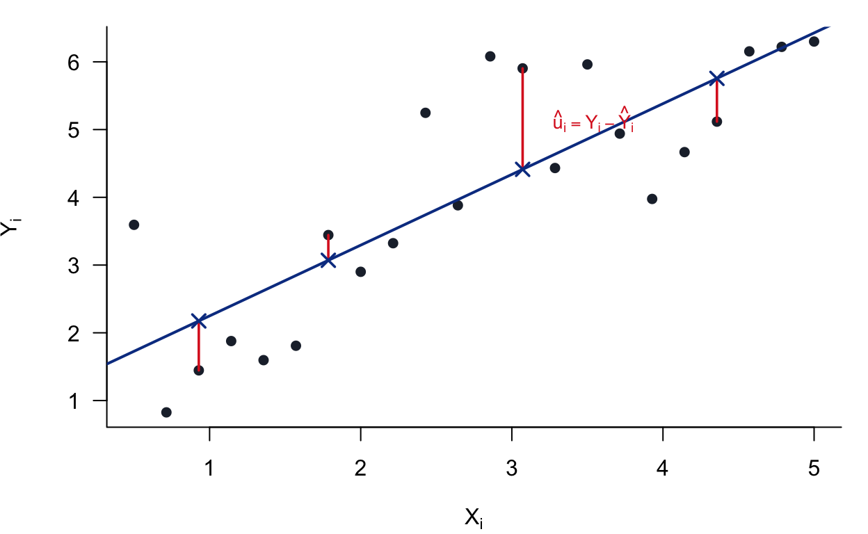
Figure 3.1: OLS minimizes the sum of squared vertical distances (red segments). The slope and intercept are chosen so no other line achieves a smaller total.
We study the simple linear regression with an intercept:
\[ Y_i = \beta_0 + \beta_1 X_i + \varepsilon_i, \qquad i = 1, \ldots, n \]
with the regularity condition \(\sum_{i=1}^n (X_i - \bar{X})^2 > 0\) (i.e., not all \(X_i\) are equal).
Sample means:
\[ \bar{Y} = \frac{1}{n} \sum_{i=1}^n Y_i, \qquad \bar{X} = \frac{1}{n} \sum_{i=1}^n X_i \]
OLS objective: Minimize the sum of squared residuals:
\[ S(\beta_0, \beta_1) = \sum_{i=1}^n \left( Y_i - \beta_0 - \beta_1 X_i \right)^2 \]
Definitions:
- Fitted values: \(\hat{Y}_i = \hat{\beta}_0 + \hat{\beta}_1 X_i\)
- Residuals: \(\hat{u}_i = Y_i - \hat{Y}_i\)
3.1.1 Derive the OLS Normal Equations
Differentiate \(S(\beta_0, \beta_1)\) with respect to \(\beta_0\) and \(\beta_1\) and set equal to zero.
First-Order Condition for \(\beta_0\):
\[ \frac{\partial S}{\partial \beta_0} = -2 \sum_{i=1}^n \left( Y_i - \beta_0 - \beta_1 X_i \right) = 0 \]
This simplifies to:
\[ \sum_{i=1}^n \left( Y_i - \beta_0 - \beta_1 X_i \right) = 0 \]
Expanding:
\[ \sum_{i=1}^n Y_i = n \beta_0 + \beta_1 \sum_{i=1}^n X_i \]
Solving for \(\beta_0\):
\[ \hat{\beta}_0 = \bar{Y} - \hat{\beta}_1 \bar{X} \]
First-Order Condition for \(\beta_1\):
\[ \frac{\partial S}{\partial \beta_1} = -2 \sum_{i=1}^n X_i \left( Y_i - \beta_0 - \beta_1 X_i \right) = 0 \]
This simplifies to:
\[ \sum_{i=1}^n X_i \left( Y_i - \beta_0 - \beta_1 X_i \right) = 0 \]
Derive the Slope in Centered Form:
Substitute \(\beta_0 = \bar{Y} - \beta_1 \bar{X}\) into the residual expression:
\[ Y_i - \beta_0 - \beta_1 X_i = Y_i - (\bar{Y} - \beta_1 \bar{X}) - \beta_1 X_i = (Y_i - \bar{Y}) - \beta_1 (X_i - \bar{X}) \]
Minimizing \(\sum_{i=1}^n \left[ (Y_i - \bar{Y}) - \beta_1 (X_i - \bar{X}) \right]^2\) with respect to \(\beta_1\) gives:
\[ \sum_{i=1}^n (X_i - \bar{X}) \left[ (Y_i - \bar{Y}) - \beta_1 (X_i - \bar{X}) \right] = 0 \]
Rearranging:
\[ \sum_{i=1}^n (X_i - \bar{X})(Y_i - \bar{Y}) = \beta_1 \sum_{i=1}^n (X_i - \bar{X})^2 \]
OLS Estimators:
\[ \boxed{\hat{\beta}_1 = \frac{\sum_{i=1}^n (X_i - \bar{X})(Y_i - \bar{Y})}{\sum_{i=1}^n (X_i - \bar{X})^2}} \]
\[ \boxed{\hat{\beta}_0 = \bar{Y} - \hat{\beta}_1 \bar{X}} \]
3.1.2 Residual Orthogonality Properties
These are the key properties that follow directly from the first-order conditions.
3.1.2.1 Residuals Sum to Zero
From the FOC for \(\beta_0\) evaluated at \((\hat{\beta}_0, \hat{\beta}_1)\):
\[ \sum_{i=1}^n \left( Y_i - \hat{\beta}_0 - \hat{\beta}_1 X_i \right) = 0 \]
Therefore:
\[ \sum_{i=1}^n \hat{u}_i = 0 \]
3.1.2.2 Residuals are Orthogonal to \(X\)
From the FOC for \(\beta_1\) evaluated at \((\hat{\beta}_0, \hat{\beta}_1)\):
\[ \sum_{i=1}^n X_i \left( Y_i - \hat{\beta}_0 - \hat{\beta}_1 X_i \right) = 0 \]
Therefore:
\[ \sum_{i=1}^n X_i \hat{u}_i = 0 \]
3.1.2.3 Residuals are Orthogonal to \((X_i - \bar{X})\)
Using the result \(\sum_{i=1}^n \hat{u}_i = 0\):
\[ \sum_{i=1}^n (X_i - \bar{X}) \hat{u}_i = \sum_{i=1}^n X_i \hat{u}_i - \bar{X} \sum_{i=1}^n \hat{u}_i = 0 - \bar{X} \cdot 0 = 0 \]
Therefore:
\[ \sum_{i=1}^n (X_i - \bar{X}) \hat{u}_i = 0 \]
3.1.2.6 Solution
Write fitted values as \(\hat Y_i=\hat\beta_0+\hat\beta_1X_i\) and expand:
\[ \sum_{i=1}^n \hat Y_i\hat u_i = \sum_{i=1}^n (\hat\beta_0+\hat\beta_1X_i)\hat u_i = \hat\beta_0\sum_{i=1}^n \hat u_i + \hat\beta_1\sum_{i=1}^n X_i\hat u_i. \]
By A1, both sums are zero. Therefore:
\[ \sum_{i=1}^n \hat Y_i \hat u_i = 0 \]
Interpretation. The part OLS explains (\(\hat Y\)) and the part it cannot explain (\(\hat u\)) do not move together in the sample.
3.1.3 Properties of Fitted Values
3.1.3.1 The Regression Line Passes Through \((\bar{X}, \bar{Y})\)
Taking the average of fitted values:
\[ \overline{\hat{Y}} = \frac{1}{n} \sum_{i=1}^n \hat{Y}_i = \frac{1}{n} \sum_{i=1}^n (\hat{\beta}_0 + \hat{\beta}_1 X_i) = \hat{\beta}_0 + \hat{\beta}_1 \bar{X} \]
Since \(\hat{\beta}_0 = \bar{Y} - \hat{\beta}_1 \bar{X}\):
\[ \overline{\hat{Y}} = (\bar{Y} - \hat{\beta}_1 \bar{X}) + \hat{\beta}_1 \bar{X} = \bar{Y} \]
Equivalently, at \(X = \bar{X}\):
\[ \hat{Y}(\bar{X}) = \hat{\beta}_0 + \hat{\beta}_1 \bar{X} = \bar{Y} \]
Conclusion: The OLS fitted line passes through the point \((\bar{X}, \bar{Y})\).
3.1.4 Decomposition of Variation (TSS = ESS + RSS)
Definitions:
| Quantity | Name | Formula |
|---|---|---|
| TSS | Total Sum of Squares | \(\sum_{i=1}^n (Y_i - \bar{Y})^2\) |
| ESS | Explained Sum of Squares | \(\sum_{i=1}^n (\hat{Y}_i - \bar{Y})^2\) |
| RSS | Residual Sum of Squares | \(\sum_{i=1}^n \hat{u}_i^2\) |
3.1.4.1 Decomposition
Start from:
\[ Y_i - \bar{Y} = (\hat{Y}_i - \bar{Y}) + (Y_i - \hat{Y}_i) = (\hat{Y}_i - \bar{Y}) + \hat{u}_i \]
Square both sides and sum:
\[ \sum_{i=1}^n (Y_i - \bar{Y})^2 = \sum_{i=1}^n (\hat{Y}_i - \bar{Y})^2 + \sum_{i=1}^n \hat{u}_i^2 + 2 \sum_{i=1}^n (\hat{Y}_i - \bar{Y}) \hat{u}_i \]
3.1.4.2 The Cross-Term Vanishes
Note that:
\[ \hat{Y}_i - \bar{Y} = (\hat{\beta}_0 + \hat{\beta}_1 X_i) - \bar{Y} = (\bar{Y} - \hat{\beta}_1 \bar{X} + \hat{\beta}_1 X_i) - \bar{Y} = \hat{\beta}_1 (X_i - \bar{X}) \]
Therefore:
\[ \sum_{i=1}^n (\hat{Y}_i - \bar{Y}) \hat{u}_i = \hat{\beta}_1 \sum_{i=1}^n (X_i - \bar{X}) \hat{u}_i = \hat{\beta}_1 \cdot 0 = 0 \]
3.1.6 Fitted Values are Orthogonal to Residuals
\[ \sum_{i=1}^n \hat{Y}_i \hat{u}_i = \sum_{i=1}^n (\hat{Y}_i - \bar{Y}) \hat{u}_i + \bar{Y} \sum_{i=1}^n \hat{u}_i = 0 + \bar{Y} \cdot 0 = 0 \]
Therefore:
\[ \sum_{i=1}^n \hat{Y}_i \hat{u}_i = 0 \]
3.1.7 Summary of Key Results
3.1.7.1 OLS Estimators
| Estimator | Formula |
|---|---|
| Slope | \(\hat{\beta}_1 = \dfrac{\sum_{i=1}^n (X_i - \bar{X})(Y_i - \bar{Y})}{\sum_{i=1}^n (X_i - \bar{X})^2}\) |
| Intercept | \(\hat{\beta}_0 = \bar{Y} - \hat{\beta}_1 \bar{X}\) |
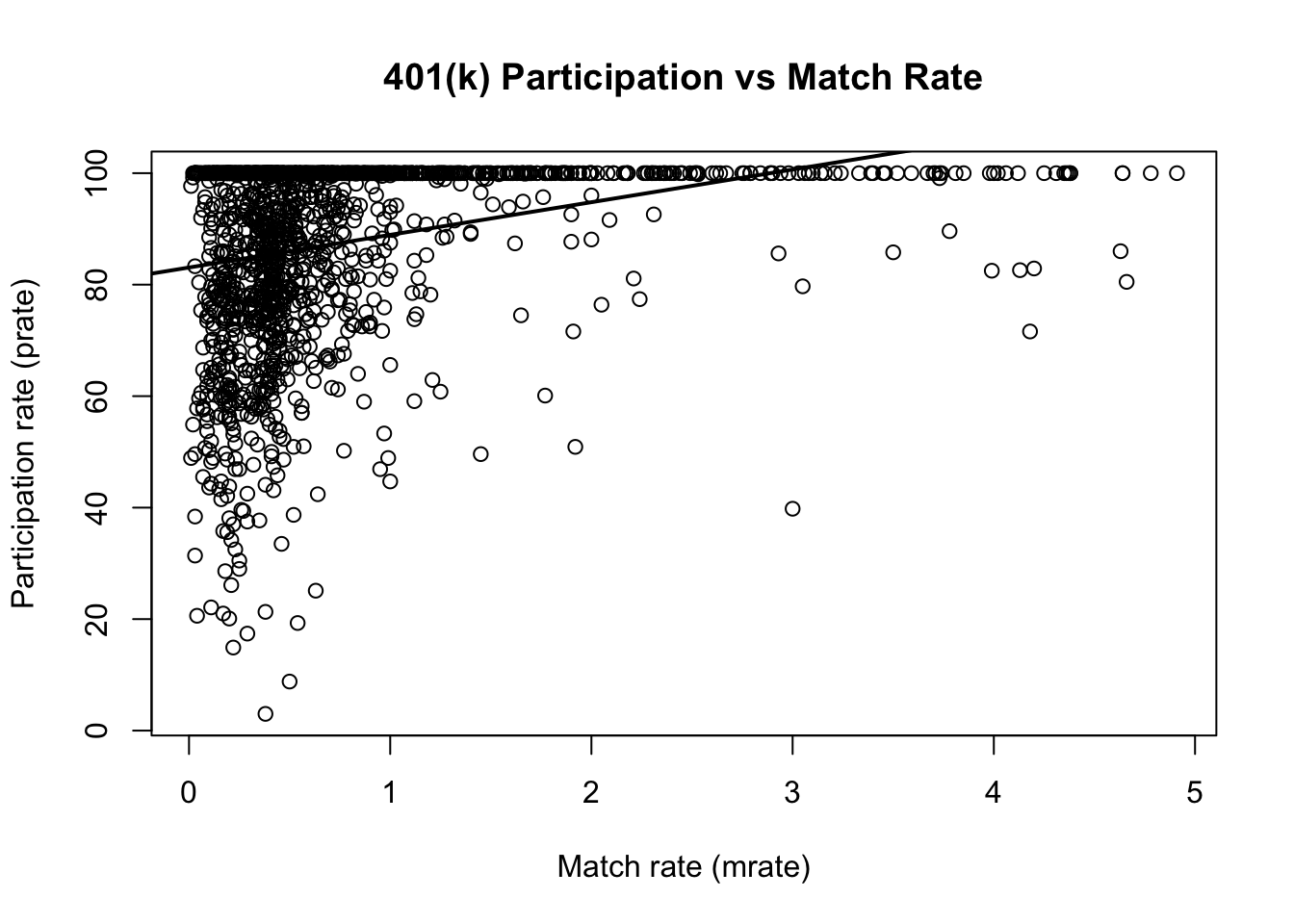
3.2 Problem 2: Wooldridge Computer Exercise C1 (401K): Participation and Match Rate
3.2.1 Overview
This notebook reproduces Wooldridge, Computer Exercise C1 (401K). Goal. Use plan-level data to study whether a more generous employer match rate is associated with higher 401(k) participation.
- Outcome:
prate= percentage of eligible workers with an active 401(k) account. - Regressor:
mrate= match rate (average firm contribution per $1 worker contribution).
We estimate the simple linear regression: \[ prate = \beta_0 + \beta_1 \, mrate + u. \]
3.2.2 Load packages and data
# If you do not have the package installed, uncomment the next line:
# install.packages("wooldridge")
library(wooldridge)

# Load the dataset used in this exercise.
data("k401k")
df <- k401k

# Quick check: dimensions and variable names
dim(df)
## [1] 1534 8
names(df)## [1] "prate" "mrate" "totpart" "totelg" "age" "totemp" "sole"
## [8] "ltotemp"3.2.3 (i) Compute the sample averages of participation and match rates
# In this dataset:
# - prate is the plan participation rate (in percentage points)
# - mrate is the match rate

mean_prate <- mean(df$prate, na.rm = TRUE)
mean_mrate <- mean(df$mrate, na.rm = TRUE)

mean_prate
## [1] 87.36291
mean_mrate## [1] 0.7315124Interpretation.
- mean_prate is the average percentage of eligible workers participating across plans.
- mean_mrate is the average employer match rate across plans.
3.2.4 (ii) Estimate the simple regression: prate on mrate
# Estimate the simple OLS regression model
m1 <- lm(prate ~ mrate, data = df)

# Summary includes coefficient estimates, standard errors, t-stats, and R^2
s1 <- summary(m1)
s1
##
## Call:
## lm(formula = prate ~ mrate, data = df)
##
## Residuals:
## Min 1Q Median 3Q Max
## -82.303 -8.184 5.178 12.712 16.807
##
## Coefficients:
## Estimate Std. Error t value Pr(>|t|)
## (Intercept) 83.0755 0.5633 147.48 <2e-16 ***
## mrate 5.8611 0.5270 11.12 <2e-16 ***
## ---
## Signif. codes: 0 '***' 0.001 '**' 0.01 '*' 0.05 '.' 0.1 ' ' 1
##
## Residual standard error: 16.09 on 1532 degrees of freedom
## Multiple R-squared: 0.0747, Adjusted R-squared: 0.0741
## F-statistic: 123.7 on 1 and 1532 DF, p-value: < 2.2e-16
# Report the sample size used by the regression (after dropping any missing values)
n <- nobs(m1)

# Extract R-squared (fraction of sample variation in prate explained by mrate)
r2 <- s1$r.squared

n
## [1] 1534
r2## [1] 0.07470313.2.5 (iii) Interpret the intercept and the slope
## (Intercept)
##    83.07546
b1## mrate
## 5.861079How to read these coefficients (economic meaning).
-
Intercept (\(\hat\beta_0\)): Predicted participation rate when
mrate = 0.- This is the fitted
pratefor a plan with no employer match. - Note: Interpretation is most meaningful if
mrate = 0is in (or near) the support of the data.
- This is the fitted
-
Slope (\(\hat\beta_1\)): Predicted change in participation (in percentage points) for a one-unit increase in
mrate.- Since
mratemeasures how many dollars the firm contributes per $1 the worker contributes, a one-unit change is economically large (e.g., from 0.5 to 1.5). - Practically, you may also interpret smaller changes:
a 0.10 increase in
mratechanges predicted participation by \(0.10 \times \hat\beta_1\).
- Since
# Example: predicted change in prate for a 0.10 increase in mrate
delta_mrate <- 0.10
pred_change_prate <- delta_mrate * b1
pred_change_prate
## mrate
## 0.58610793.2.6 (iv) Predicted participation when mrate = 3.5. Is it reasonable?
# Prediction at mrate = 3.5
pred_35 <- predict(m1, newdata = data.frame(mrate = 3.5))
pred_35
## 1
## 103.5892To assess whether this prediction is reasonable, check whether mrate = 3.5 lies within the observed range of the data.
Predictions far outside the support of mrate are extrapolations, which can be unreliable.
# Range of mrate in the sample
range_mrate <- range(df$mrate, na.rm = TRUE)
range_mrate
## [1] 0.01 4.91
# Also helpful: a few quantiles to understand typical values
quantile(df$mrate, probs = c(0, .05, .25, .5, .75, .95, 1), na.rm = TRUE)
## 0% 5% 25% 50% 75% 95% 100%
## 0.0100 0.1100 0.3000 0.4600 0.8300 2.3635 4.9100Discussion prompt (what is happening if it looks unreasonable):
- If 3.5 is much larger than typical match rates in the data, then the fitted value is based on
extending a linear trend beyond where you have information.
- In addition, prate is a percentage and should generally lie between 0 and 100; a linear model can
produce fitted values outside this range, especially under extrapolation.
3.2.7 (v) How much of the variation in prate is explained by mrate?
The share of variation in prate explained by mrate in this simple model is the R-squared:
r2## [1] 0.0747031Interpretation. - \(R^2\) is the fraction of sample variation in participation that is accounted for by variation in the match rate. - Whether it is “a lot” depends on context; in cross-sectional data, modest \(R^2\) values are common.